Statistics has become significantly popular in the recent years with the exponential growth in the applications in various fields like Economics, Business, Healthcare, Logistics, Risk Management, Policy Making, Government Institutions and every possible industry where data is generated. Data is the new oil, with the application of blend of cutting edge technologies and Statistical Methods we can solve most complex business problems. With the advent of Big Data, Machine Learning and Artificial Intelligence, majority of the companies are incorporating data analytics and data driven solutions when building strategic applications and decision making.
What is Statistics?
‘Statistics is a branch of applied mathematics which specializes in
data.’ - This is the
most straightforward yet simple definition of statistics.
Definitions by Great Statisticians:
1. "Statistics is the science of counting. The
science of averages." - A.L. Bowley
2. "Statistics is the science of Estimates and
Probabilities" – Boddington
3. "Statistics is the science and art of handling
aggregates of facts – observing, enumeration, recording, classifying and
otherwise systematically treating them" – Harlow
These are
few of many definitions of Statistics which are changing by time.
In these series of blogs I'll be sharing the important statistical concepts and methods that are using in the present day Machine Learning Projects.
Let's now look into the Data Types that we use in the Statistics.
Types of Data
We generally
face two types of data in our machine learning projects:
1.
Numerical Data
2. Categorical Data
Numerical
Data: Numerical
data again classified into two types -
1. Discrete data – which assumes only integer
values just like int variable.
Example: Age of a person,
Number of Subjects passed in a semester,
Number of Children in a family, etc.
2. Continuous data - which assumes integer as well
as decimal values just like float
variable.
Example: Height and weight of a person,
Average speed of your car trip,
Temperature in a room, etc.
Categorical
Data: Unlike numerical
data, categorical data doesn’t have any numerical values to represent the data,
it rather uses “Names” or “Labels”. Categorical data is again divided into two
types:
1. Nominal Data – In Nominal Data, the Names/Labels
are non-measurable and all have equal importance, no Label is placed higher or
No Label is placed lower, all are ranked same. (We cannot put labels on a scale
and measure them)
Example: a) What is your gender?
You either choose “Male” or “Female”,
here two Names/Labels are equally ranked. No Label has the priority over the other.
(Or we cannot measure the gender)
b) In grammar, the parts of speech:
Noun, Verb, Preposition, Article, Pronoun, etc.
(we cannot measure the parts of speech)
2. Ordinal
Data – In Ordinal Data, the Names/Labels are measurable and are ranked on the
Ordinal Scale. (you often see these as rating scales in different applications)
Example: a) If an order is delivered to
you, and asked to give the rating for their service on a scale of 1-10. 1 being very poor and 10 being
Fantastic.
(Here we are measuring their service
on a scale.)
b) How is your Coffee? - Very Strong,
Strong, Moderate, Light, Very Light.
(Here we are measuring the taste of a
coffee.)
Presenting the data in the descriptive from is the foremost step in any Statistical Analysis or building a Machine Learning model. It gives insights on the data that we are working on and allows us to spot any patterns in the data.
Descriptive Statistics
Measures of Central Tendency
Mean: Arithmetic Mean or simply the Mean is defined as the sum of the observations divided by the number of observations.
Output: 16.2
Median: The Median is that value which divides the data into two equal parts, one part comprising all values greater, and the other, all values lower than Median.
Output: 17
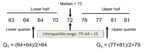
Quartiles: The Quartiles divide the given data into four parts. There are three quartiles. The second quartile divides the data into two halves and therefore is the same as the Median. The first (lower) quartile (Q1) marks off the first one-fourth, the third (upper) quartile (Q3) marks off the three-fourth.
Inter-Quartile Range: It is defined as the difference between the third (upper) quartile (Q3) and the first (lower) quartile (Q1).
Interquartile Range = Q3-Q1
Quartile Deviation: It is half of the difference between the first (lower) quartile (Q1) and the third (upper) quartile (Q3). Hence, it is called Semi Inter Quartile Range.
Quartile Deviation = (Q3-Q1)/2

 |
Mode: The Mode refers to that value in the data, which occur most frequently. It is an actual value, which has the highest concentration of items in and around it.
Measures of Dispersion
Mean Deviation: Mean Deviation is the arithmetic mean of the deviations of a series computed from any measure of central tendency; i.e, Mean, Median and Mode. All the deviations are taken as positive i.e, signs are ignored.
According to Clark and Schekade: "Average deviation is the average amount scatter of the items in a distribution from either the mean or the median, ignoring the signs of the deviations."
We usually compute mean deviation from any one of the three averages, Median is most preferred over others. But in general practice and due to wide applications of mean, the mean deviation is generally computed from mean.
Standard Deviation: Karl Pearson introduced the concept of Standard Deviation in 1893. It is the most important measure of dispersion and is widely used in many statistical formulae. Standard Deviation is also called as Root-Mean Square Deviation (Error)[RMSE], which is the most important metric we use while checking the fit of our Machine Learning Regression models.
Definition: "It is defined as the positive square-root of the arithmetic mean of the square of the deviations of the given data from their arithmetic mean."
Variance: Square of the Standard Deviation is called Variance.

Comments
Post a Comment